Kenneth McAfee

Expectation value, expected value, EV, <x>: they all mean the same thing. At the highest level, expectation value measures a sort of weighted average: given outcomes (a, b, c) with associated probabilities (P(a), P(b), P(c)), for a given scenario, what would we expect our “average” outcome to be.

Taking a look at the different ways people would try and gain an edge on the books, I kept coming across the use of expectation value. This wasn’t overtly surprising; sports betting is a statistical exercise, so it would make sense for these concepts to have a home in betting strategies. However, I began to feel like the essence of expectation value and statistics overall was being lost in favor of punchlines to the tune of “positive expectation value = cash in your pocket!” While I don’t believe this saying is necessarily wrong, I think keeping the statistical flavor of expectation value in its application to sports betting can become a powerful tool for looking at the bigger picture. In the following sections, I hope to provide an overview of what expectation value is, how it fits into statistical systems, and how it governs the outcomes of a book and its customers.

Definition

I think it will prove useful to start with the general definition of expectation value. Note that <> brackets denote expectation value for a certain variable. So, for a given bet, the expected value for net profit, , can be expressed as:

This tells us that the expectation value for any given bet depends solely on how a book sets a line relative to the actual projected odds. Being able to accurately predict odds and set a line accordingly is the crux of how a sports book can become so profitable. However, professional sports are inherently dynamic—lines can move up and down drastically before an event and no one model is able to predict probabilities with 100% certainty.

“Positive EV” strategists attempt to target discrepancies between the odds a book might set and the actual odds of an outcome, and in doing so place a wager with a positive expectation value. These ‘actual odds’ are a bit of a black box, however. I won’t pretend to have the secret sauce for predicting games, but throughout my PhD I’ve done a fair bit of uncertainty quantification and can demonstrate how these systems play out, so let’s figure out what this looks like.

Simulating Statistical Systems

To simulate statistical systems, we can use a technique called Monte Carlo analysis to project the behavior of different betting strategies out to 10, 100, or 100,000 samples. One important thing to note before we dive into the weeds: this type of analysis will not give a deterministic outcome, but rather a distribution of outcomes. Being able to properly digest a Monte Carlo or other statistical simulation is just as important as running the simulation itself. See FiveThirtyEight’s prediction of the 2016 presidential election, for example.

So, let’s say a book is setting the line for the Superbowl coin toss. The odds here are a predictable 50/50, but lines set at +100/+100 will never be profitable for the book. 50/50 lines will typically be set at -110/-110, for reasons we are about to see. From our definition above this gives us . Predicting what our net profit will look like if we bet $1 on heads over the next 100 Superbowls is fairly straight forward. For each coin flip, we have a 50% chance of either gaining $0.91, or losing $1. Propagating this forward 100 times gives us something like this.

Unsurprisingly, we have a negative net profit. But, this doesn’t really tell us much, only one possible scenario. To really look at our outlook, we need to repeat this a few times say, 20.

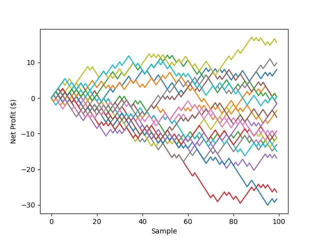
In the above plot, each colored line represents an independent trial of 100 coin flips. This data recovers some of the “randomness” we would expect, but we’re still not in the realm of statistical significance. The are, however, some general qualitative behaviors coming though at this point:

1. In most trial runs, there is a net loss after 100 samples.
2. Bets with negative expectation value can lead to a profit. Conversely, and more importantly when considering risk, bets with positive expectation value can lead to a loss.

Let’s keep repeating the same set of simulations to see what happens when we drastically increase the number of 100 coin flip trials, e.g. 10,000.

Looking at the above chart we can see how the cluster of repeat trials forms a non-trivial distribution of outcomes. If we take a slice of the profits after 100 coin flips the results can then be visualized as a distribution.

This distribution encodes all the information about the upsides and downsides for a given betting strategy used over only a relatively small number of attempts. For starters, note that the average net profit over 100 coin flips is approximately -$4.5, which lines up right with our expectation value of -4.5%. So, over a significant number of trials, our average net return is equivalent to the expectation value of that bet. The width of the distribution encodes information about the odds of bets placed. For a betting strategy which prioritizes generally unfavorable outcomes (odds < 50%), the distribution will broaden, increasing potential winnings while also amplifying exposure to large losses. The inverse is true for strategies favoring probable outcomes, where potential winnings are trimmed down in favor of a much more palatable downside. I will save the specifics of this for a different post, but the main takeaway here should be as follows: as an individual bettor, your net outcome is a distribution which is governed by the expectation value and odds of your wagers.

The Book vs. The Bettors

From the book’s perspective, we have to look at it in a slightly different fashion. While individual bettors may place only tens or hundreds of bets in any significant time period, the book’s are issuing millions of wagers per day between hundreds of events. For them, statistical significance is reached easily and their outcomes take on a more deterministic form. If we return to the canonical coin flip example, it becomes easy to see how quickly the net return converges on 4.5% in a relatively short time period. Let’s say the book issues 500 bets per day with the same odds as before and a of +4.5% (Note how is positive now because we’re looking at things from the book’s perspective). We can simulate this scenario as we did before, shown in the figure below repeated 5 times. The solid black line shows the trend for a 4.5% return on each bet.

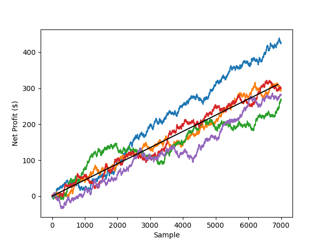
Over a 2 week time span (500 bets/day x 14 days = 7000 samples), it can be seen how each of the 5 simulations converge to a similar trend. In statistics, this would be a demonstration of the Law of Large Numbers. In essence, sample size is the engine behind how a sports book can generate so much profit and why, as a bettor, there is no surefire method to coming out ahead without a significant time investment. When a book issues a series of wagers at a given expectation value, the very nature of the outcome is different depending on which side you look at it from.

From the individual bettor’s perspective, the net outcome is a distribution, not any given value. The sample size is not statistically significant.

From the book’s perspective, the net outcome is a predictable value due to the aggregation of individual wagers creating a statistically significant sample size.

So, in the end, to actually make money sports betting one needs to both figure out 1) how to predict odds better than the books, and 2) get lucky. The smaller the sample size, the more important luck becomes, even with a positive expectation value. So next time someone tells you they make money sports betting… they might be telling the truth, but the odds are not in their favor.